Count single mitochondrial DNA nucleoids and quantify mitochondrial network volume
Expected run time for this demo: few minutes.
In this tutorial we will count the number of mitochondrial DNA nucleoids and we will segment the mitochondrial network in 3D as a reference channel.
For details about the method used to visualize these structures see this publication.
Goals
Detect and separate highly connected spots
Segment network-like structures as reference channel (mitochondrial network)
Filter valid spots based on reference channel signal
Preliminary steps
The first step with every new dataset is to segment the objects. These typically are the single cells, but it can be any object where you want to detect spots.
While you can detect spots in the entire image, it is highly recommended to identify region of interests (ROIs) and segment them.
The dataset provided with this tutorial already contains the segmentation files with the ROIs of the single cells, but if you need to segment ROIs we recommend using out other software called Cell-ACDC.
Dataset
To follow this tutorial, download the dataset from here.
This dataset was published in this publication.
After unzipping the downloaded file, you will see the following folder structure:
Position_26
└── Images
    ├── ASY15-1_0nM-26_s26_acdc_output.csv
    ├── ASY15-1_0nM-26_s26_last_tracked_i.txt
    ├── ASY15-1_0nM-26_s26_metadata.csv
    ├── ASY15-1_0nM-26_s26_mKate.tif
    ├── ASY15-1_0nM-26_s26_mNeon.tif
    ├── ASY15-1_0nM-26_s26_phase_contr.tif
    ├── ASY15-1_0nM-26_s26_segm.npz
    └── ASY15-1_0nM-26_s26_segmInfo.npz
Some of these files are generated by Cell-ACDC and they will not be discussed here.
What we can see is that we have 3 .tif files corresponding to 3 channels
whose filename end with mKate.tif, mNeon.tif, phase_contr.tif.
The phase_contr channel is the channel we used to segment the single cells with
Cell-ACDC. The resulting segmentation masks are saved in the file ending with
segm.npz.
The mNeon channel is the channel where we want to detect the spots.
The mKate channel is the labelling of the mitochondrial network and we can
use it in SpotMAX as the reference channel (more details below).

A) Phase contrast channel used for segmentation of the cells. B) mNeon channel used to visualize the mitochondrial DNA nucleoids (spots channel). Arrows indicate areas of connected spots. C) mKate channel used to label the mitochondrial network (reference channel).
Tip
SpotMAX can take advantage of mother-bud (or sister cells) relationships. To
annotate the relationship use the Cell-ACDC software. These annotations
are saved in the file ending with acdc_output.csv.
Loading the dataset
Now that we have our dataset with the segmentation file of the cells, we can proceed with detecting the spots.
Important
In this tutorial we assume that you are already familiar with the analysis parameters. If not, please read about them here: Description of the parameters.
Click on the 
Load folder button on the top-right of the GUI.
Select the Position_26 folder you downloaded and load the mNeon channel.
When the dataset is loaded, you will see on the Analysis parameters tab on the left that some of the parameters have already been filled out.
Now let’s see how we can determine the optimal parameters for this dataset.
Setting up the parameters
The parameters are grouped into separate sections so we will go one by one.
File paths and channels
Since we want to segment the mitochondrial network as a reference channel from
the mKate channel, we write ‘mKate’ in the Reference channel end name parameter.
If we want to take advantage of the mother-bud (or sister cells) pairings we write
‘acdc_output.csv’ in the Table with lineage info end name parameter.
We can then decide on a Run number (in this case we leave it at 1), and,
optionally, we can append a text at the end of the output files, for example we
could write ‘tutorial’ at in the Text to append at the end of the output files.
Finally, we select ‘.csv’ for the File extension of the output tables.
METADATA
Since some of the metadata is already saved in the file ending with metadata.csv
some of the entries were correctly loaded.
We need to correct the Spots reporter emmission wavelength (nm) to
509 since the fluorescence probe used to image the mitochondrial DNA is mNeonGreen.
Now we need to determine the optimal values for the
Spot minimum z-size (μm) and Resolution multiplier in y- and x- direction
parameters. These are important because if the resulting
Spot (z, y, x) minimum dimensions (radius) is too low we will detect
multiple peaks within the same spot. On the other hand, if it is too high, we
risk to miss the smaller spots. For this tutorial we will use
Spot minimum z-size (μm) = 1.0 and
Resolution multiplier in y- and x- direction = 2.0.
Tip
The simplest way to determine these values is to use the tools available
in the Tune parameters tab. See more instructions in this section
Tune parameters tab and here Spot minimum z-size (μm).
Once you have inserted these values you should now see the following at the
Spot (z, y, x) minimum dimensions (radius) parameter:
Spot (z, y, x) minimum dimensions (radius)  (1.0, 0.4357, 0.4357) μm
                                            (2.8571, 6.479, 6.479) pxl
Pre-processing
For the pre-processing activating or not the Aggregate cells prior analysis
will not make any difference becasue we are working with a single mother-daughter
pair. If we would be working with multiple cells and we already know that some
of the cells in the image do not have spots activating this parameter might
be very important (especially if we use Thresholding for the
Spots segmentation method).
We do not need to activate Remove hot pixels because this specific
dataset does not have any very bright isolated single pixel.
We leave the Initial gaussian filter sigma to 0.75 because we want to
activate Sharpen spots signal prior detection. When sharpening is active,
the gaussian filtered image is not used for detection but only for quantification.
Using a small gaussian sigma is recommended to remove some of the background
noise. With a higher sigma the smoothing would be to aggressive, especially
because we are dealing with low signal-to-noise ratio.
Tip
You can visually inspect the result of every pre-processing filter
by pressing on the  compute button beside each filter.
Reference channel
In this tutorial, as well as detecting the spots, we also want to segment the
mitochondrial network from the mKate signal as the reference channel.
We will then use the resulting segmentation to remove those spots that are
outside of the mitochondrial network (we are interested in detecting only the
mitochondrial DNA that is inside the mitochondrial network).
To this purpose we activate Segment reference channel.
Another important parameter we want to activate is Use the ref. channel mask to determine background.
This is because we want to keep only those spots that are significantly brighter
than the mKate signal in the same area. However, we cannot compare absolute
intensities between mNeon and mKate because they are two different
fluorophores. Therefore, we need to normalize the two signals before comparing
them. To do so, SpotMAX will divide the mean of the signal within each spot
(using the minimum spot size determined in the metadata_mtdna_yeast_tutorial
section) by the background median. To determine the background, we want to take
the median of the pixels that are outside of the spots, but inside of the
mitochondrial network, hence we activate this parameter.
Next, we turn our attention onto the filters that are available to enhance
the segmentation accuracy. Since we are dealing with network-like structures,
a gaussian filter (smoothing) might not be enough. A better filter in this case
is a ridge operator. These operators take one or more values called sigmas
used as scales of the filter. For this specific dataset, we write 2, 3 in the
Sigmas used to enhance network-like structures parameter.
Tip
Selecting the right sigmas for the ridge operator might require some trial
and error. Some values that you can test are 1, 2, 1, 2, and
2, 3. The more sigmas you use, the longer the computation time.
Test these values by both visually inspecting the result of the filter and
the result of the segmentation (using the compute buttons).
For the Ref. channel gaussian filter sigma parameter instead, we leave
this one at 0.75 to remove some background noise.
Now we need to choose whether to use the ‘Thresholding’ or ‘BioImage.IO model’
for the Ref. channel segmentation method. Since we know that
‘Thresholding’ works well in this case we will use that, but feel free to
experiment with any of the models available at the BioImage Model Zoo.
Next, to choose the optimal Ref. channel threshold function we click
on the button beside the Ref. channel segmentation method
and we should be able to appreciate that thresholding_yen, threshold_otsu,
and threshold_isodata all do a pretty good job at segmenting the mitochondrial
network. We will proceed with thresholding_yen.
Finally, we can choose whether to Save reference channel segmentation masks
and Save pre-processed reference channel image.
Spots channel
We are almost done, since this is the last section that we will setup.
For the Spots segmentation method we know that ‘SpotMAX AI’ works
well in this case, but feel free to experiment with ‘Thresholding’ (which is much faster
than the neural networks) and with any of the models available at the BioImage Model Zoo.
Note
If this is the first time you are using the ‘SpotMAX AI’ method, SpotMAX will need to install some libraries. Keep an eye on the terminal during this time and check that installation is successful.
After selecting ‘SpotMAX AI’ you will need to configure the parameters of the
model. To do so, click on the  cog button beside the parameter. If you
want more information about the parameters of the AI see this section
SpotMAX AI parameters. For this dataset, we know that the following parameters
work well:
cog button beside the parameter. If you
want more information about the parameters of the AI see this section
SpotMAX AI parameters. For this dataset, we know that the following parameters
work well:
Model type: 2D
Preprocess across experiment: False
Preprocess across timepoints: False
Gaussian filter sigma: 0.0
Remove hot pixels: False
Config yaml filepath: SpotMAX_v2/spotmax/nnet/config.yaml
PhysicalSizeX: 0.0672498 (same as in the metadata_mtdna_yeast_tutorial)
Resolution multiplier yx: 1.0
Next, we can ignore Spot detection threshold function because we
are using the ‘SpotMAX AI’ method.
Now, as we said at the beginning, we want to keep only those spots that are
significantly higher than the reference channel in the same place. To do so,
we can take advantage of a couple of features to filter valid spots. One
way to compare the two signals is to perform a Welch’s t-test and keep only
those spots whose p-value of the test is below a certain threshold. Therefore
at the Features and thresholds for filtering true spots we click on
the Set features or view the selected ones button and we expand the
Statistical test (vs. ref. ch.) group. We then select the p-value (t-test) feature
and we click Ok. Next, we select a maximum bound for the p-value of 0.025.
Since this would result in keeping those spots whose mean intensity is both
significantly and lower then the reference channel, to keep only those that have
higher mean intensity we click on the 
Add feature button and we
add the t-statistic from the Statistical test (vs. ref. ch.) group. Finally,
we set a minimum bound on the t-statistic of 0, meaning that we will
keep only those spots whose mean intensity is higher than the reference channel.
Here is how the window to select the features should look like:
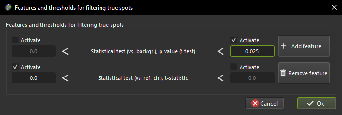
Window used to select features and thresholds for filtering true spots.
We now activate Optimise detection for high spot density, and we do
not activate Compute spots size (fit gaussian peak(s)).
Finally, we can choose whether to Save spots segmentation masks and
Save pre-processed spots image.
Note
Since we do not activate Compute spots size (fit gaussian peak(s))
we do not need to worry about the paramters in the SpotFIT
section. Also, we can leave the Configuration section deactivated
and we will get asked about it when we run the analysis
Running the analysis
Ok, we are finally ready to run the analysis!
To do so simply click on the 
Run analysis... button on the top
right of the tab.
SpotMAX will now allow use to save the parameters to an INI configuration file
and we choose ‘Yes’. This way we can load them back into the GUI any time we
want by clicking on the Load parameters from previous analysis...
button on the top-left of the tab.
Next, SpotMAX will ask us whether we want to select the measurements to save and we say ‘No, save all the measurements’.
Then we choose a filename for the parameters file and the folder where to save them. We will get a dialogue confirming that parameters where saved with the path where they have been saved. We click ‘Ok’ and we get a reminder that the analysis will now run in the terminal and we should keep an eye on that.
We click on ‘Ok, run now!’ and we move our attention to the terminal. In the terminal we will get asked some last questions about parameters that we did not selected and we simply confirm that we want to use the default ones.
The analysis will now run and the output files will be saved in the
same folder of the dataset in a new folder called SpotMAX_output. For details
about the output files see this section Output files.
Closing remarks
At the end of the analysis you can go back to the GUI and visualize and inspect the results using the tools in the Inspect and edit results.
That’s it! I hope you found this tutorial useful and you can let us know if you found mistakes or any other feedback on our GitHub page or by sending us an email at .
Until next time!